If you’ve been following my blog, I like to use R and ggplot2 for data visualization. A lot.
One of my older blog posts, An Introduction on How to Make Beautiful Charts With R and ggplot2, is still one of my most-trafficked posts years later, and even today I see techniques from that particular post incorporated into modern data visualizations on sites such as Reddit’s /r/dataisbeautiful subreddit.
However, that post is a little outdated. Thanks to a few updates to ggplot2 since then and other advances in data visualization best-practices, making pretty charts for websites/blogs using R and ggplot2 is even more easy, quick, and fun!
Quick Introduction to ggplot2
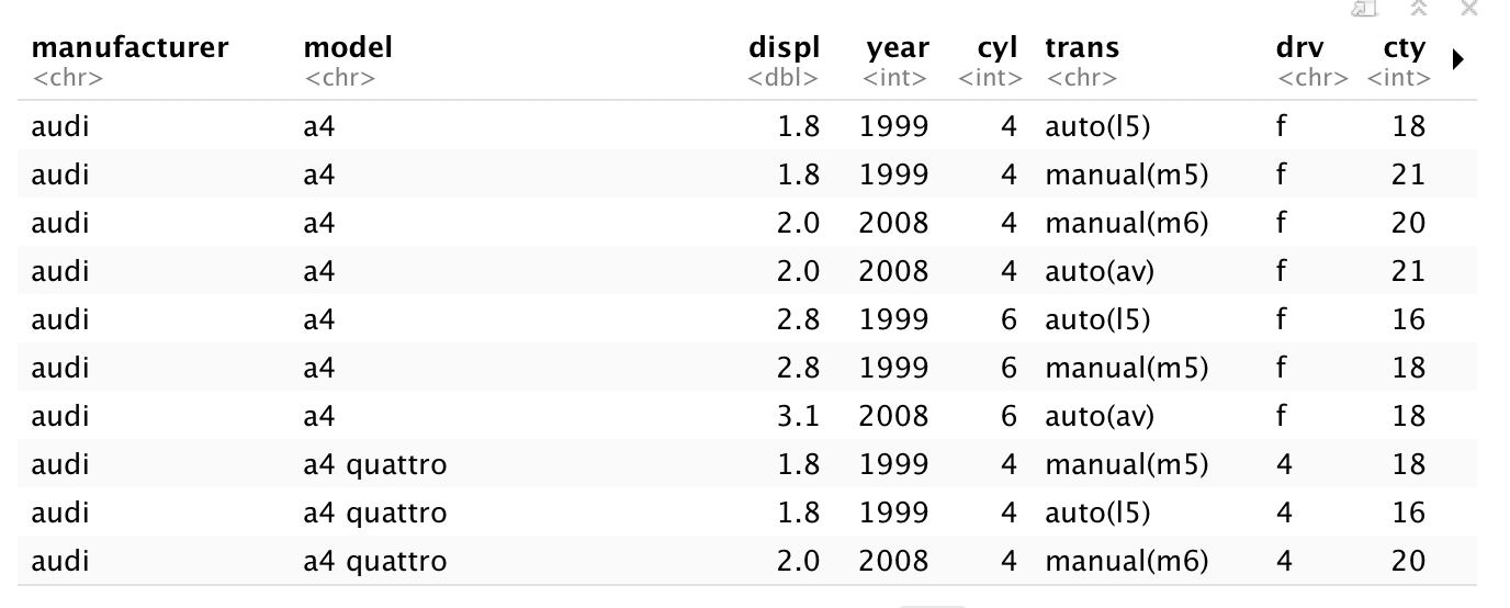
ggplot2 uses a more concise setup toward creating charts as opposed to the more declarative style of Python’s matplotlib and base R. And it also includes a few example datasets for practicing ggplot2 functionality; for example, the mpg dataset is a dataset of the performance of popular models of cars in 1998 and 2008.
Let’s say you want to create a scatter plot. Following a great example from the ggplot2 documentation, let’s plot the highway mileage of the car vs. the volume displacement of the engine. In ggplot2, first you instantiate the chart with the ggplot() function, specifying the source dataset and the core aesthetics you want to plot, such as x, y, color, and fill. In this case, we set the core aesthetics to x = displacement and y = mileage, and add a geom_point() layer to make a scatter plot:
p <- ggplot(mpg, aes(x = displ, y = hwy)) +
			geom_point()
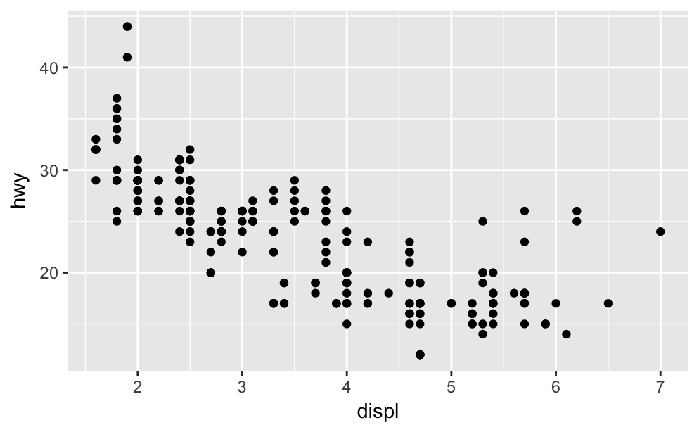
As we can see, there is a negative correlation between the two metrics. I’m sure you’ve seen plots like these around the internet before. But with only a couple of lines of codes, you can make them look more contemporary.
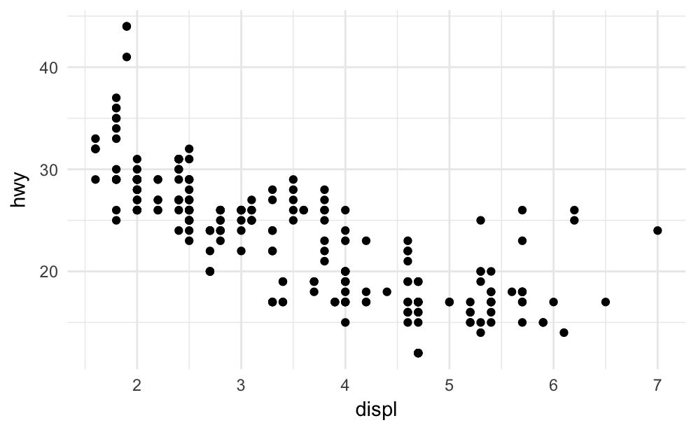
ggplot2 lets you add a well-designed theme with just one line of code. Relatively new to ggplot2 is theme_minimal(), which generates a muted style similar to FiveThirtyEight’s modern data visualizations:
p <- p +
    theme_minimal()
But we can still add color. Setting a color aesthetic on a character/categorical variable will set the colors of the corresponding points, making it easy to differentiate at a glance.
p <- ggplot(mpg, aes(x = displ, y = hwy, color=class)) +
			geom_point() +
			theme_minimal()
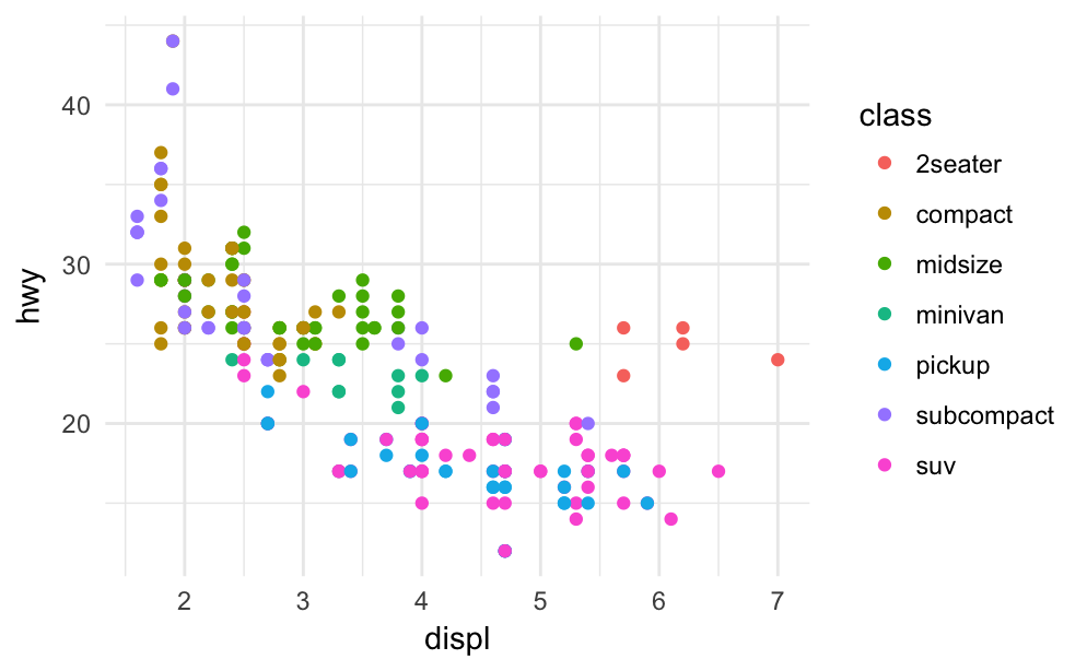
Adding the color aesthetic certainly makes things much prettier. ggplot2 automatically adds a legend for the colors as well.
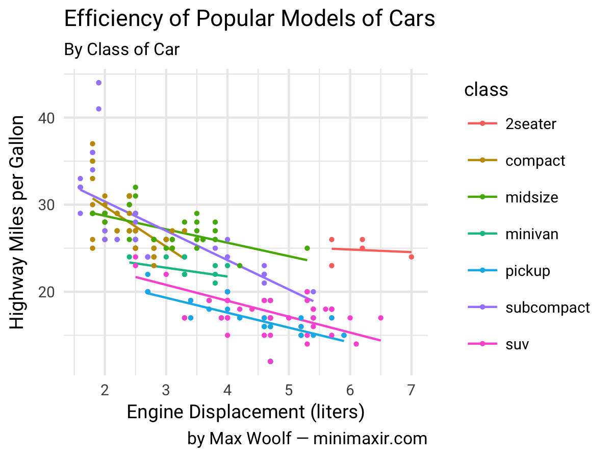
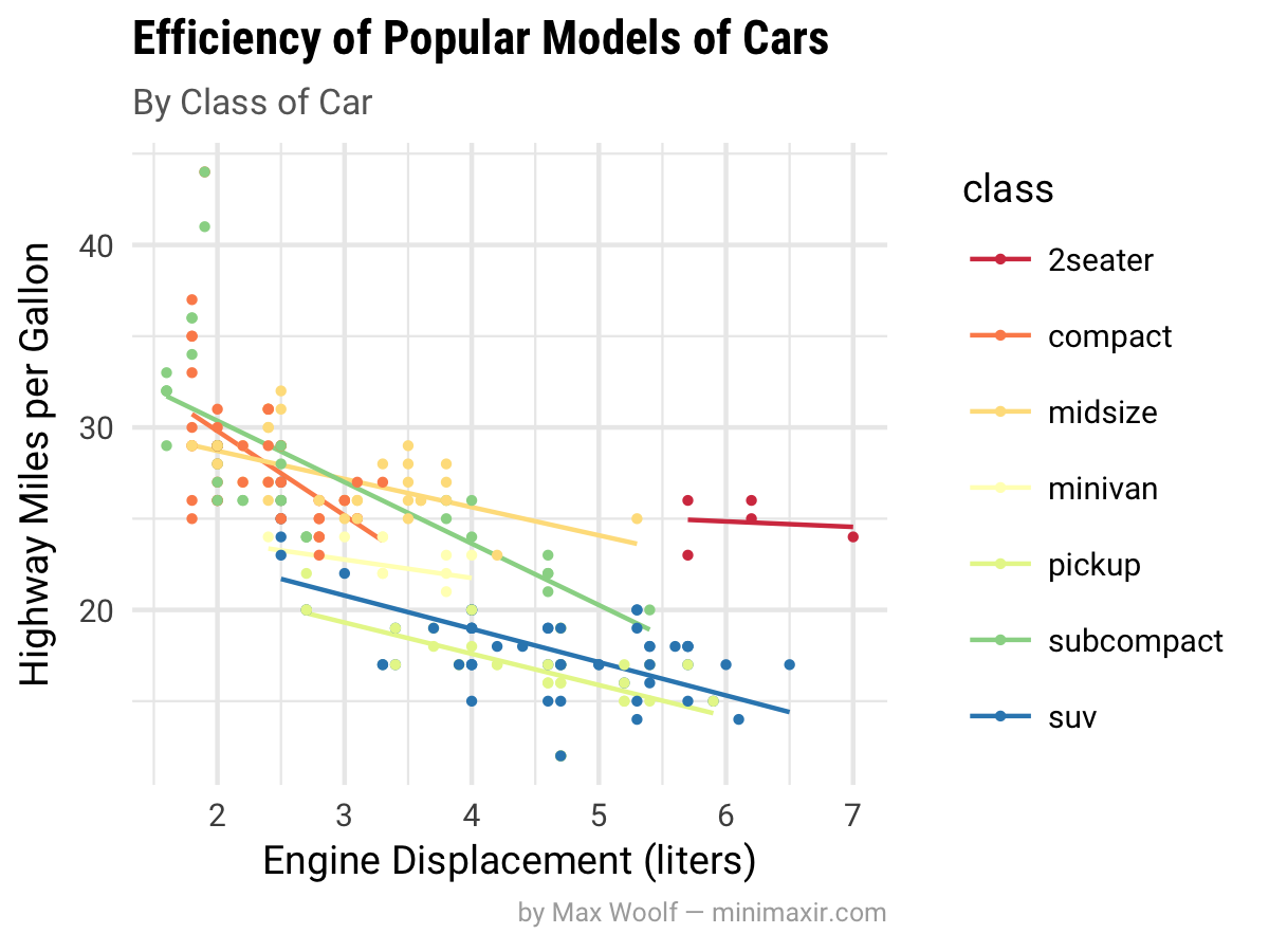
However, for this particular visualization, it is difficult to see trends in the points for each class. A easy way around this is to add a least squares regression trendline for each class using geom_smooth() (which normally adds a smoothed line, but since there isn’t a lot of data for each group, we force it to a linear model and do not plot confidence intervals)
p <- p +
	geom_smooth(method = "lm", se = F)
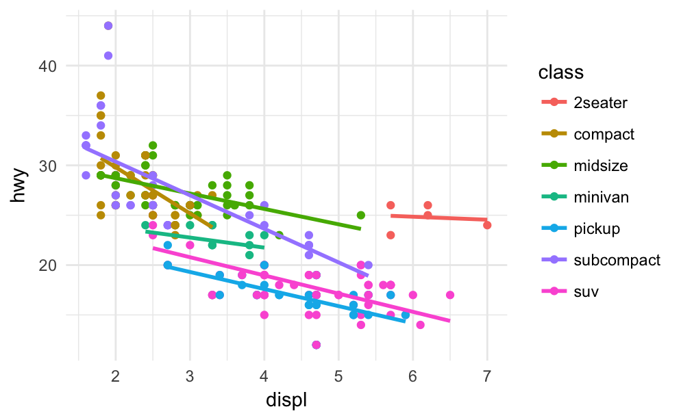
Pretty neat, and now comparative trends are much more apparent! For example, pickups and SUVs have similar efficiency, which makes intuitive sense.
The chart axes should be labeled (always label your charts!). All the typical labels, like title, x-axis, and y-axis can be done with the labs() function. But relatively new to ggplot2 are the subtitle and caption fields, both of do what you expect:
p <- p +
    labs(title="Efficiency of Popular Models of Cars",
         subtitle="By Class of Car",
         x="Engine Displacement (liters)",
         y="Highway Miles per Gallon",
         caption="by Max Woolf — minimaxir.com")
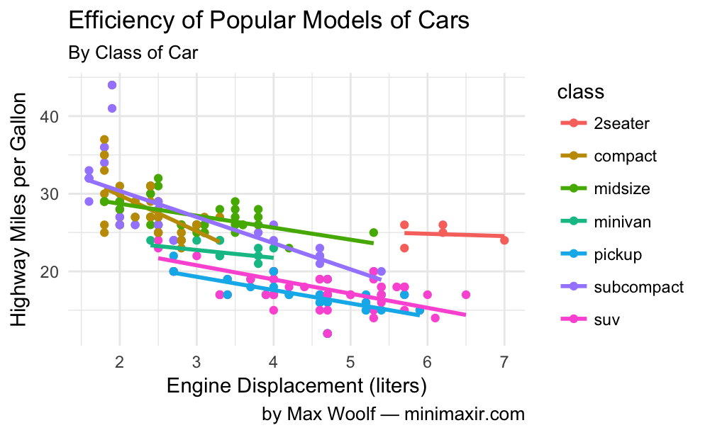
That’s a pretty good start. Now let’s take it to the next level.
How to Save A ggplot2 chart For Web
Something surprisingly undiscussed in the field of data visualization is how to save a chart as a high quality image file. For example, with Excel charts, Microsoft officially recommends to copy the chart, paste it as an image back into Excel, then save the pasted image, without having any control over image quality and size in the browser (the real best way to save an Excel/Numbers chart as an image for a webpage is to copy/paste the chart object into a PowerPoint/Keynote slide, and export the slide as an image. This also makes it extremely easy to annotate/brand said chart beforehand in PowerPoint/Keynote).
R IDEs such as RStudio have a chart-saving UI with the typical size/filetype options. But if you save an image from this UI, the shapes and texts of the resulting image will be heavily aliased (R renders images at 72 dpi by default, which is much lower than that of modern HiDPI/Retina displays).
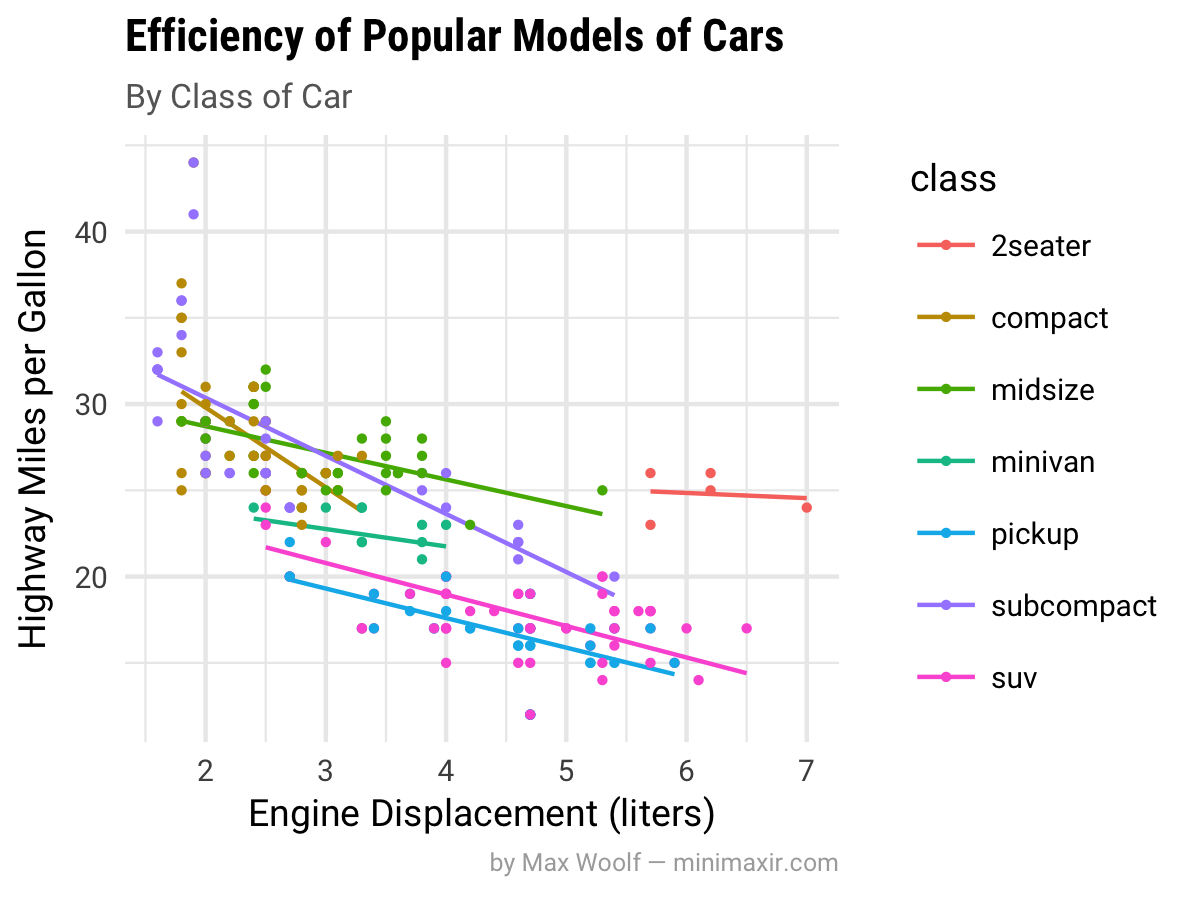
The data visualizations used earlier in this post were generated in-line as a part of an R Notebook, but it is surprisingly difficult to extract the generated chart as a separate file. But ggplot2 also has ggsave(), which saves the image to disk using antialiasing and makes the fonts/shapes in the chart look much better, and assumes a default dpi of 300. Saving charts using ggsave(), and adjusting the sizes of the text and geoms to compensate for the higher dpi, makes the charts look very presentable. A width of 4 and a height of 3 results in a 1200x900px image, which if posted on a blog with a content width of ~600px (like mine), will render at full resolution on HiDPI/Retina displays, or downsample appropriately otherwise. Due to modern PNG compression, the file size/bandwidth cost for using larger images is minimal.
p <- ggplot(mpg, aes(x = displ, y = hwy, color=class)) +
    geom_smooth(method = "lm", se=F, size=0.5) +
    geom_point(size=0.5) +
    theme_minimal(base_size=9) +
    labs(title="Efficiency of Popular Models of Cars",
         subtitle="By Class of Car",
         x="Engine Displacement (liters)",
         y="Highway Miles per Gallon",
         caption="by Max Woolf — minimaxir.com")

ggsave("tutorial-0.png", p, width=4, height=3)
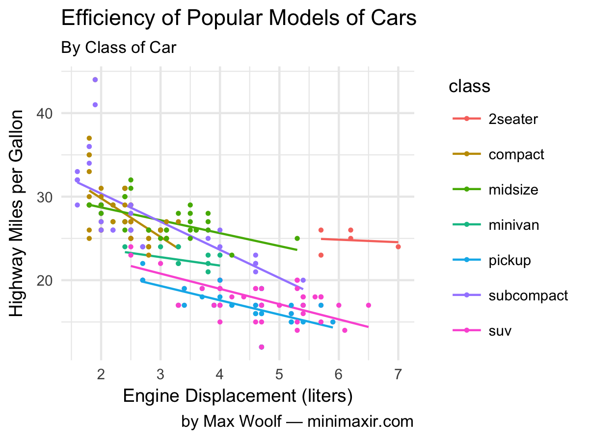
Compare to the previous non-ggsave chart, which is more blurry around text/shapes:
For posterity, here’s the same chart saved at 1200x900px using the RStudio image-saving UI:
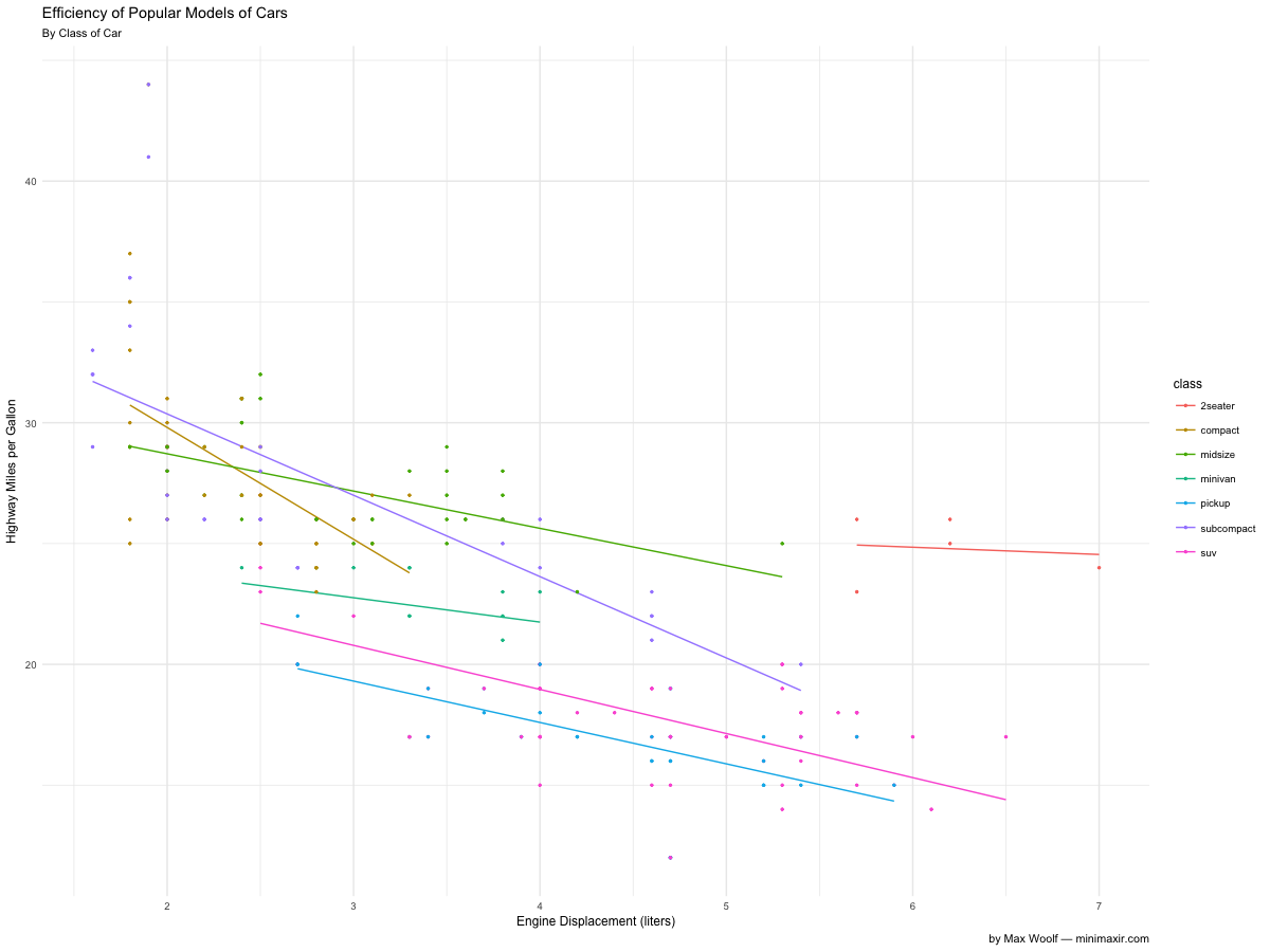
Note that the antialiasing optimizations assume that you are not uploading the final chart to a service like Medium or WordPress.com, which will compress the images and reduce the quality anyways. But if you are uploading it to Reddit or self-hosting your own blog, it’s definitely worth it.
Fancy Fonts
Changing the chart font is another way to add a personal flair.
Theme functions like theme_minimal() accept a base_family parameter. With that, you can specify any font family as the default instead of the base sans-serif. (On Windows, you may need to install the extrafont package first). Fonts from Google Fonts are free and work easily with ggplot2 once installed. For example, we can use Roboto, Google’s modern font which has also been getting a lot of usage on Stack Overflow’s great ggplot2 data visualizations.
p <- p +
    theme_minimal(base_size=9, base_family="Roboto")
A general text design guideline is to use fonts of different weights/widths for different hierarchies of content. In this case, we can use a bolder condensed font for the title, and deemphasize the subtitle and caption using lighter colors, all done using the theme() function.
p <- p +
    theme(plot.subtitle = element_text(color="#666666"),
          plot.title = element_text(family="Roboto Condensed Bold"),
          plot.caption = element_text(color="#AAAAAA", size=6))
It’s worth nothing that data visualizations posted on websites should be easily legible for mobile-device users as well, hence the intentional use of larger fonts relative to charts typically produced in the desktop-oriented Excel.
Additionally, all theming options can be set as a session default at the beginning of a script using theme_set(), saving even more time instead of having to recreate the theme for each chart.
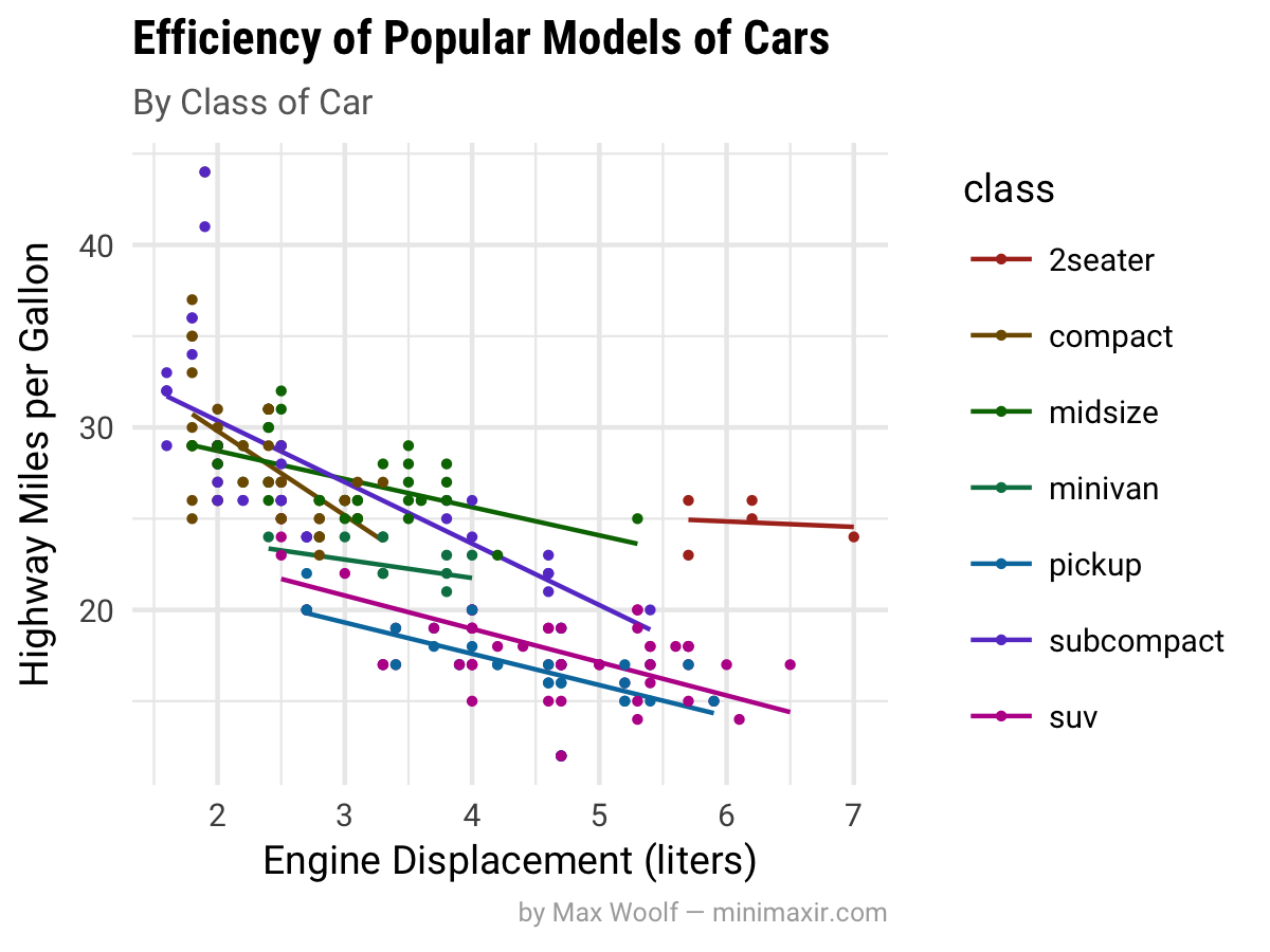
The “ggplot2 colors”
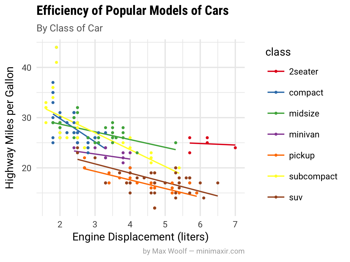
The “ggplot2 colors” for categorical variables are infamous for being the primary indicator of a chart being made with ggplot2. But there is a science to it; ggplot2 by default selects colors using the scale_color_hue() function, which selects colors in the HSL space by changing the hue [H] between 0 and 360, keeping saturation [S] and lightness [L] constant. As a result, ggplot2 selects the most distinct colors possible while keeping lightness constant. For example, if you have 2 different categories, ggplot2 chooses the colors with h = 0 and h = 180; if 3 colors, h = 0, h = 120, h = 240, etc.
It’s smart, but does make a given chart lose distinctness when many other ggplot2 charts use the same selection methodology. A quick way to take advantage of this hue dispersion while still making the colors unique is to change the lightness; by default, l = 65, but setting it slightly lower will make the charts look more professional/Bloomberg-esque.
p_color <- p +
        scale_color_hue(l = 40)
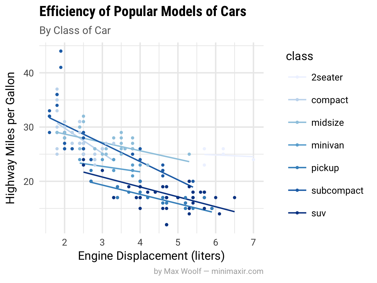
RColorBrewer
Another coloring option for ggplot2 charts are the ColorBrewer palettes implemented with the RColorBrewer package, which are supported natively in ggplot2 with functions such as scale_color_brewer(). The sequential palettes like “Blues” and “Greens” do what the name implies:
p_color <- p +
        scale_color_brewer(palette="Blues")
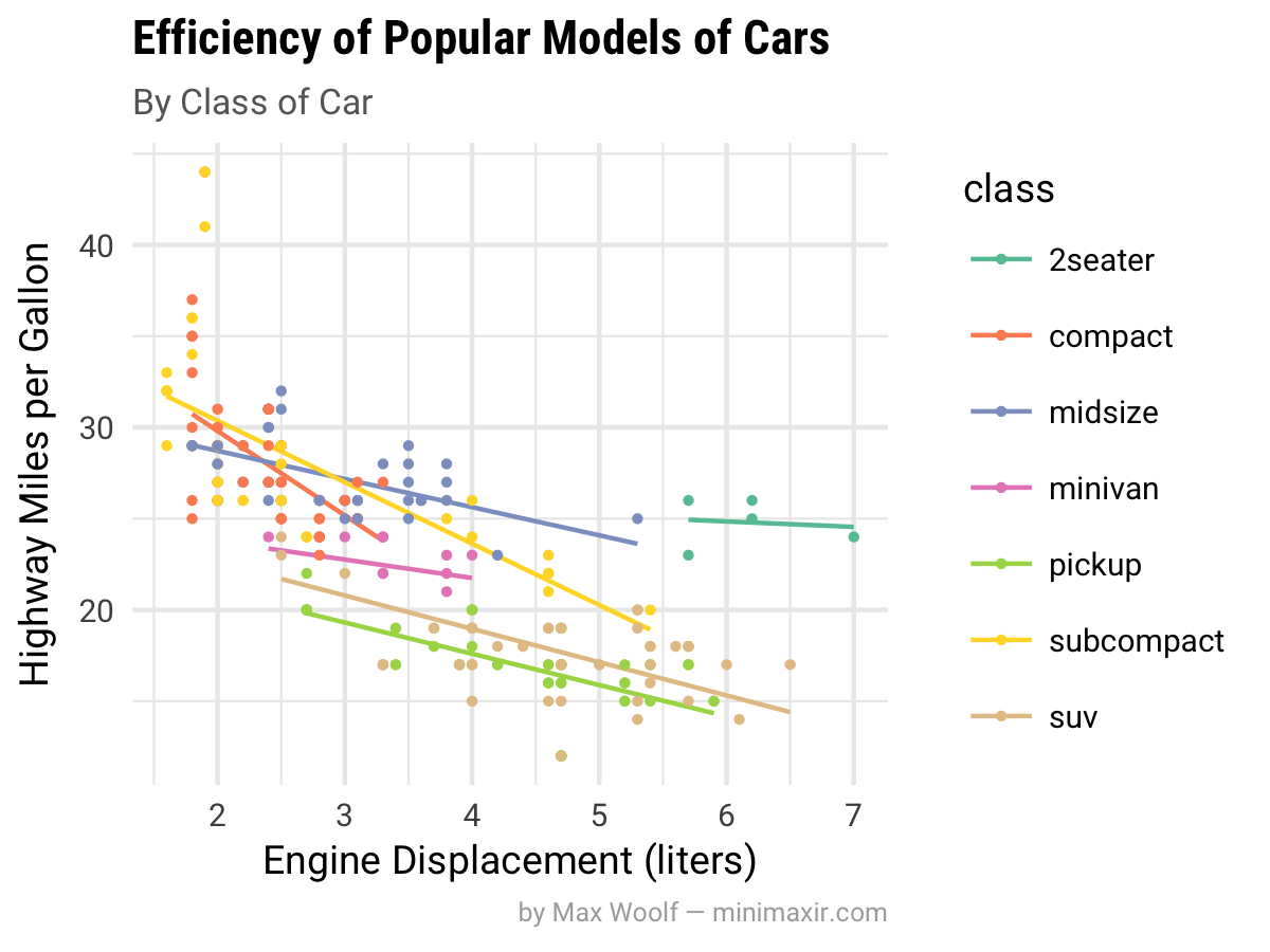
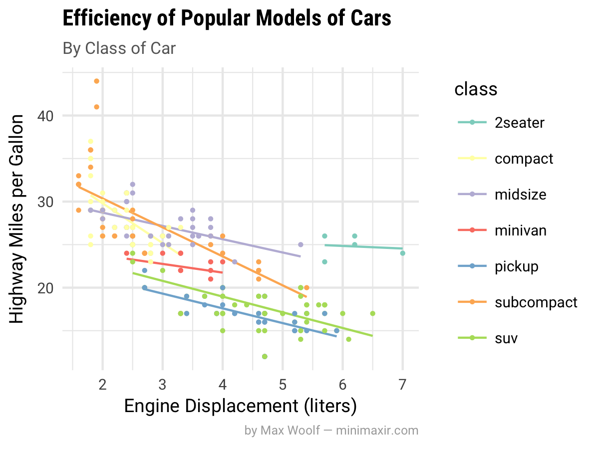
A famous diverging palette for visualizations on /r/dataisbeautiful is the “Spectral” palette, which is a lighter rainbow (recommended for dark backgrounds)
However, while the charts look pretty, it’s difficult to tell the categories apart. The qualitative palettes fix this problem, and have more distinct possibilities than the scale_color_hue() approach mentioned earlier.
Here are 3 examples of qualitative palettes, “Set1”, “Set2”, and “Set3,” whichever fit your preference.
Viridis and Accessibility
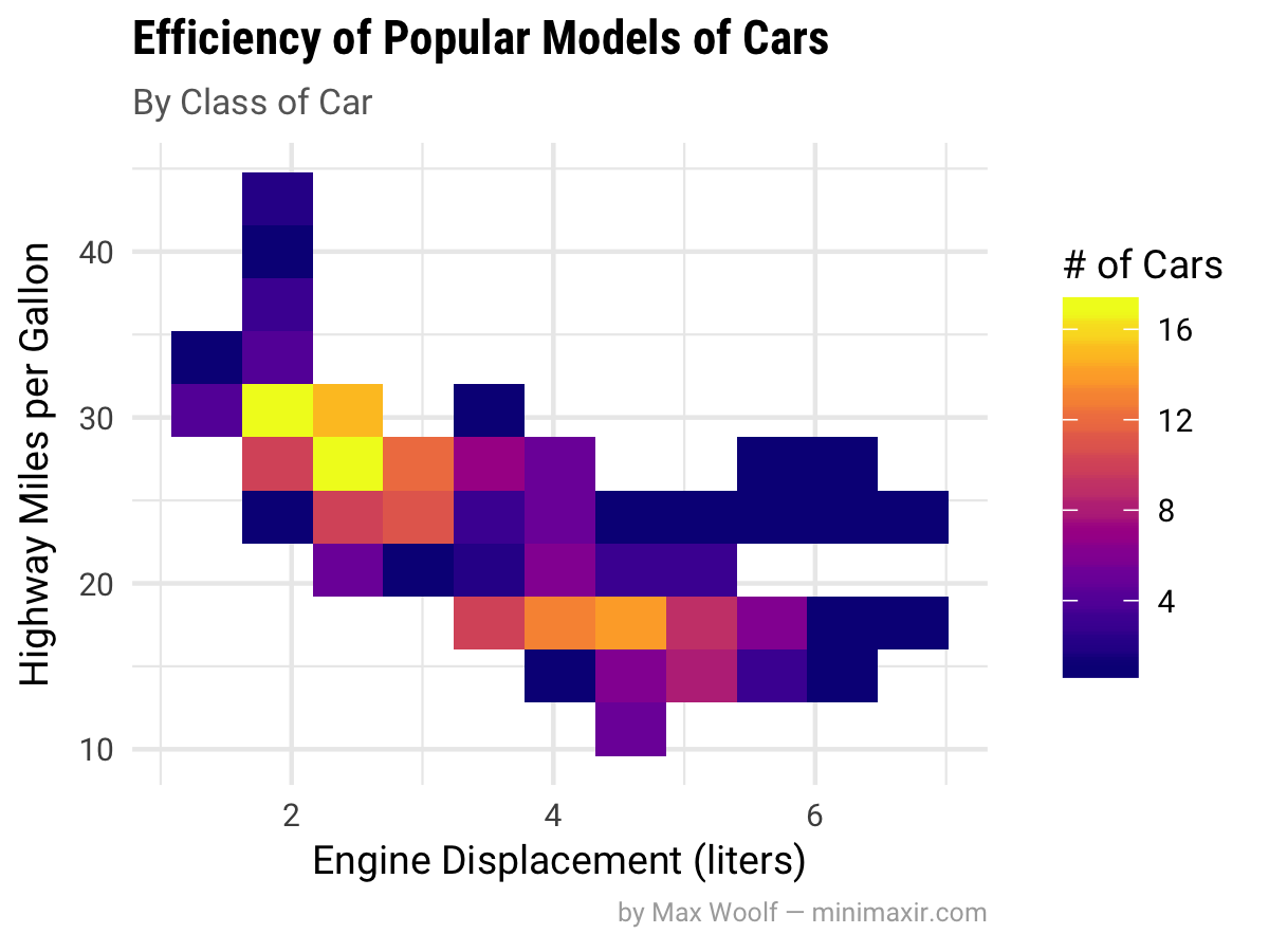
Let’s mix up the visualization a bit. A rarely-used-but-very-useful ggplot2 geom is geom2d_bin(), which counts the number of points in a given 2d spatial area:
p <- ggplot(mpg, aes(x = displ, y = hwy)) +
    geom_bin2d(bins=10) +
    [...theming options...]
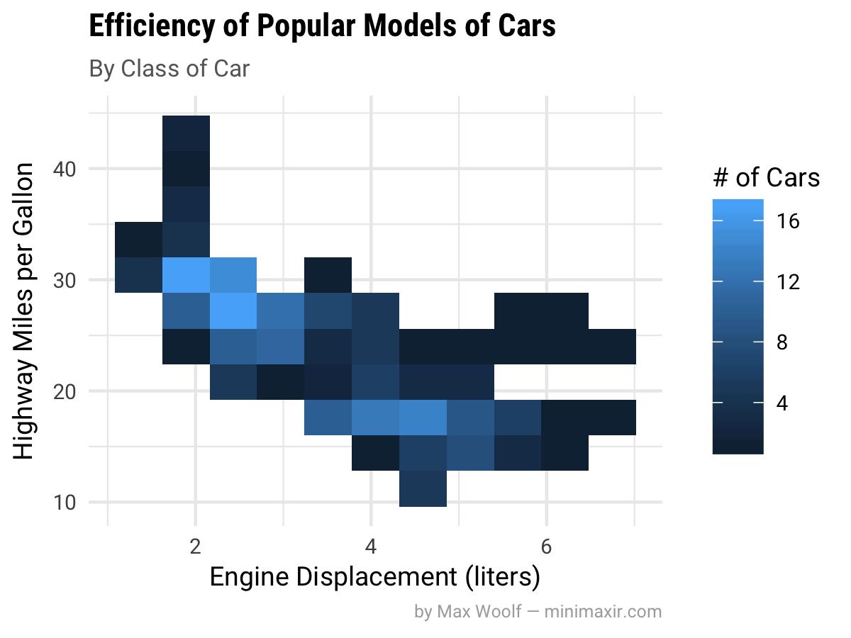
We see that the largest number of points are centered around (2,30). However, the default ggplot2 color palette for continuous variables is boring. Yes, we can use the RColorBrewer sequential palettes above, but as noted, they aren’t perceptually distinct, and could cause issues for readers who are colorblind.
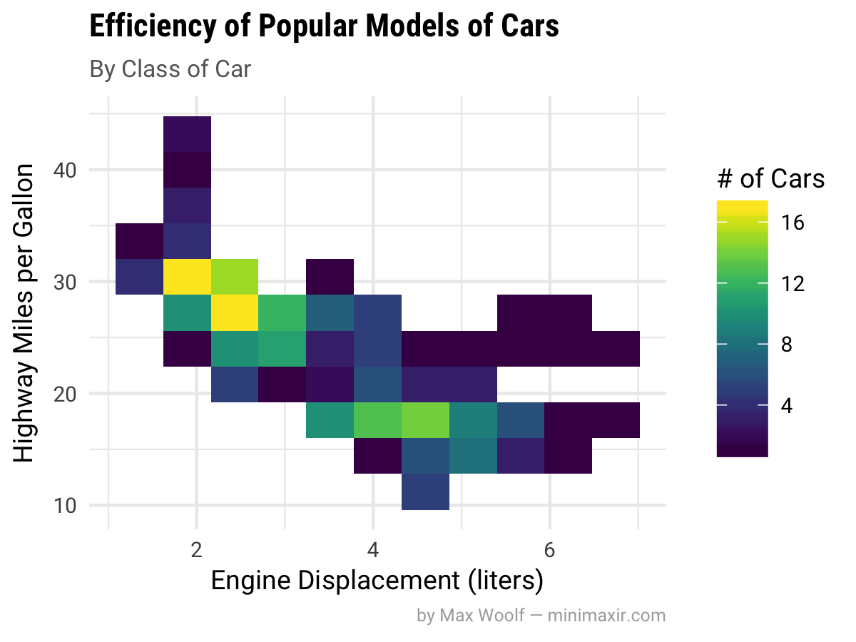
The viridis R package provides a set of 4 high-contrast palettes which are very colorblind friendly, and works easily with ggplot2 by extending a scale_fill_viridis()/scale_color_viridis() function.
The default “viridis” palette has been increasingly popular on the web lately:
p_color <- p +
        scale_fill_viridis(option="viridis")
“magma” and “inferno” are similar, and give the data visualization a fiery edge:
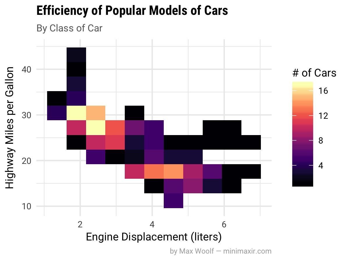
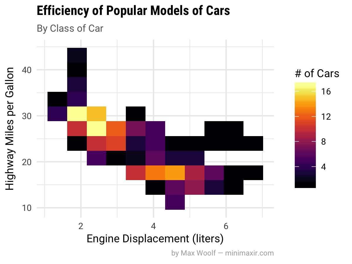
Lastly, “plasma” is a mix between the 3 palettes above:
Next Steps
FiveThirtyEight actually uses ggplot2 for their data journalism workflow in an interesting way; they render the base chart using ggplot2, but export it as as a SVG/PDF vector file which can scale to any size, and then the design team annotates/customizes the data visualization in Adobe Illustrator before exporting it as a static PNG for the article (in general, I recommend using an external image editor to add text annotations to a data visualization because doing it manually in ggplot2 is inefficient).
For general use cases, ggplot2 has very strong defaults for beautiful data visualizations. And certainly there is a lot more you can do to make a visualization beautiful than what’s listed in this post, such as using facets and tweaking parameters of geoms for further distinction, but those are more specific to a given data visualization. In general, it takes little additional effort to make something unique with ggplot2, and the effort is well worth it. And prettier charts are more persuasive, which is a good return-on-investment.
You can view the R and ggplot2 code used to create the data visualizations in this R Notebook. You can also view the images/data used for this post in this GitHub repository.
You are free to use the data visualizations from this article however you wish, but it would be greatly appreciated if proper attribution is given to this article and/or myself!